Single Trial EEG Data Analysis and BVAtoR
Sarah von Grebmer
25 April 2020
basic-usage.RmdThe BVAtoR package takes segmented output from BVA (.dat files, .vmrk files and .vhdr files) and transforms them into a single file with all voltage values, participants, conditions, and other variables specified by the experimenter for further single trial statistical analysis. This vignette describes the installation and use of the package in order to obtain a (large) dataframe containing EEG data from BVA output.
BVAtoR Pre-Requisites
This package works excusively with BVA (V2.2) export files, i.e. pre-processed, segmented and baseline-corrected data (not averaged data). An important step during segmentation in BVA is to assign the resulting node a meaningful name, ideally containing information about the participant (i.e. participant number) and the condition, separated by underscores (or any other separator).
Upon termination of the classical pre-processing procedure (e.g. re-referencing, filtering, ocular correction, artefact rejection, segmentation, baseline correction) in BVA, the data is ready for export. Note that each condition for each participant will have to be exported separately. See below for instructions on how to export data from BVA.
Exporting Data from BVA
In BVA, select the node from which you want to export data, namely the baseline corrected node containing information about single trials.
In BVA, click EXPORT/GENERIC DATA/ tick WRITE HEADER FILE and WRITE MARKER FILE/ select TEXT FORMAT for the header and marker file/include participant number and condition in the basename (CRUCIAL!)/ click NEXT
Select TEXT FORMAT as data file format/MULTIPLEXED as data orientation/ LINE DELIMITERS as PC format/ click NEXT
Tick ADD CHANNEL NAMES TO THE DATAFILE/ Tick OVERWRITE DEFAULT DECIMAL SYMBOL (,) and replace to DOT/CUSTOM PRECISION TO SIX OR MORE/ change value layout to SEPARATE VALUES BY CUSTOM SEPARATOR/ set separator to semi-colon (;)/ click NEXT
Untick EXPORT ALL CHANNELS/ remove VEOG, HEOG AND ALL EYE CHANNELS from selected channels / click FINISH
This will create three separate export files in your EXPORT folder. Make a copy of these files and copy all files to a separate folder, which will be the working directory of this current pipeline.
- dat file: contains the voltage values for each channel
- vmrk file: markers text file that contains the order of appearance of the markers and their timestamp in samples
- vhdr file: header file which contains metadata such as sampling frequency and the link between the two other export files
Note: Example File Name To illustrate the naming of files, the file subj100_comp_BaselineCorrection_cogn_incongr_nonviol.dat contains the following information:
subj100: subject number comp: Name of Task Baseline_Correction: Node of export in BVA (i.e. exported after baseline correction before averaging) cogn: Level 1 of Condition 1 congr: Level 1 of Condition 2 non-viol: Level 1 of Condition 3
BVAtoR Package
The BVAtoR package was specifically created to combine the voltage values in the .dat file with the information about the markers in the .vmrk file to generate a large datafile that contains the variables “marker” and “voltage”, among other variables, such as condition etc.
# Load package
library(BVAtoR)
BVA_to_R() parameters
BVAtoR is based on a number of helper functions which tackle the formatting of the export files and the extraction of crucial information, such as the sampling frequency or the marker names. The helper functions run in the background of the core function of this package, the BVA_to_R() function. Please see below for a more detailed description of the helper functions. The core function takes a number of parameters that should be known to the researcher prior to starting this analysis:
path: path to the data folder with all exort files, e.g. “template/path/to/all/files/” . Specified outside the main function.
full_window_bounds: The total length of the exported segment in ms (e.g. c(-200, 1200). Specified within the main function.
ERP_list: List of ERP components of interest with their associated lower and upper time limits. These should correspond to the time windows of the ERP component sand cover the entire segment. See below for an example. Specified outside the main function.
Note: Ensure to cover the entire length of the segment. Prior to setting ERP time limits, the researcher must be aware of the number of time samples taken during the duration of a segment and the sampling rate. The sampling frequency (SF) in Hz is needed to calculate this time interval, and can be retrieved from the .vhdr file.
If we assume a sampling frequency (SF) of 500Hz the time inbetween voltage samples (in milliseconds ms) is calculated as follows:
1000 ms/SF = Time_Increment 1000 ms/500 = Time_Increment 1000 ms/500 = 2 ms
This reads as: at a sampling frequency of 500 Hz, voltage is measured every 2 ms. Now we need to calculate the number of voltage samples per segment
To calculate the number of voltage samples taken during a segment of (for example) 1400 ms:
Total_segment_Length in ms/ Time_Increment = Number_of_Samples 1400 ms/2 ms = 700 voltage samples
In conclusion, the time bounds for each ERP component cannot be odd numbers. See below for an example. Further parameters to be specified are:
var_labs : variables to inlcude as columns in the final datafile. These correspond to the information given in the exported data file names, i.e. participant, condition etc. Specified within the main function.
sep: specifies the separator with which the variables within the exported data file names are separated by. Specified within the main function.
filename_returned: the name of the file to be returned in csv format, e.g. “Output.csv”. Contains columns for subject, marker, condition (if applicable), timestamp, ERP component (if applicable), node of segmentation, task (if applicable) etc. for further single trial statisitical analysis in R. Specified within the main function.
BVA_to_R() usage
# Help to main function
#?BVA_to_R

# Specify path to export files
path <- "../inst/extdata/"

# Specify list of ERPs (example), ensure to cover entire window length and that they do not overlap
ERPs <- list(
  "baseline" = c(-200, 48), # pre-stimulus
  "N100" = c(48, 198),
  "P200" = c(200, 348),
  "N400" = c(350, 498),
  "P600" = c(500, 898), # longer P600 window for late learners (example-specific)
  "PostP600" = c(900, 1198) # end of segment
)

# Call main function and generate final datafile (obj)
obj <- BVA_to_R(
  path = path,
  sep = "_",
  ERP_list = ERPs,
  var_labs = c("Subject", "Comp", "Export_Node",
               "Cognate_Status", "Congruency_Type", "Violation_Type"),
  full_window_bounds = c(-200, 1198)
)

head(obj)
#>    time posit_datapoints    Fp2     F8    FT8     T8    TP8    P8   TP10    O2
#> 1: -200                1 -5.132 -1.770 -0.219  2.732  4.565 9.213 -0.862 5.375
#> 2: -198                2 -4.047 -1.380 -0.543  1.518  3.966 8.941 -1.495 5.183
#> 3: -196                3 -2.915 -0.598 -0.586  0.341  3.340 8.509 -2.036 4.824
#> 4: -194                4 -1.929  0.565 -0.241 -0.690  2.540 7.840 -2.474 4.314
#> 5: -192                5 -1.137  2.049  0.470 -1.532  1.387 6.862 -2.753 3.662
#> 6: -190                6 -0.454  3.722  1.395 -2.203 -0.185 5.550 -2.844 2.874
#>        Oz     O1    TP9      P7    TP7     T7    FT7     F7    FP1    AFz
#> 1:  1.354 -4.257 -4.016 -14.087 -9.069 -4.742 -2.709 -2.273 -2.221 -4.558
#> 2:  0.686 -4.748 -4.816 -14.161 -9.707 -5.096 -1.484 -1.914 -2.004 -3.674
#> 3: -0.021 -5.079 -5.803 -13.910 -9.935 -4.933 -0.084 -1.125 -1.570 -2.402
#> 4: -0.713 -5.215 -6.734 -13.386 -9.775 -4.346  1.267  0.002 -0.953 -0.918
#> 5: -1.306 -5.088 -7.392 -12.635 -9.298 -3.473  2.356  1.351 -0.233  0.646
#> 6: -1.741 -4.658 -7.595 -11.668 -8.576 -2.447  2.999  2.770  0.496  2.209
#>        F4    FC4     C4    CP4     P4    Pz     P3    CP3     C3   FC3     F3
#> 1: -7.670 -6.508 -7.184  0.137  5.398 3.268 -6.575 -2.973 -1.974 0.263 -1.932
#> 2: -6.318 -6.081 -7.493 -0.881  4.971 3.407 -5.853 -2.190 -0.900 1.233 -1.061
#> 3: -4.613 -5.246 -7.682 -2.129  4.117 3.333 -4.973 -1.258  0.424 2.549  0.324
#> 4: -2.791 -4.202 -7.906 -3.652  2.822 2.982 -4.077 -0.305  1.794 3.980  2.005
#> 5: -1.008 -3.099 -8.238 -5.452  1.139 2.343 -3.261  0.567  3.003 5.314  3.724
#> 6:  0.683 -1.993 -8.625 -7.431 -0.807 1.475 -2.548  1.291  3.897 6.392  5.244
#>        Fz    FCz   CPz    Cz descrip marker_num posit_onset      ERP Subject
#> 1: -3.884 -1.142 3.987 3.794    S189        Mk2         101 baseline kons104
#> 2: -2.557  0.476 4.463 4.931    S189        Mk2         101 baseline kons104
#> 3: -0.682  2.514 4.854 6.143    S189        Mk2         101 baseline kons104
#> 4:  1.466  4.651 5.037 7.242    S189        Mk2         101 baseline kons104
#> 5:  3.666  6.611 4.915 8.039    S189        Mk2         101 baseline kons104
#> 6:  5.754  8.201 4.450 8.394    S189        Mk2         101 baseline kons104
#>    Comp        Export_Node Cognate_Status Congruency_Type Violation_Type
#> 1: comp BaselineCorrection        noncogn         incongr        nonviol
#> 2: comp BaselineCorrection        noncogn         incongr        nonviol
#> 3: comp BaselineCorrection        noncogn         incongr        nonviol
#> 4: comp BaselineCorrection        noncogn         incongr        nonviol
#> 5: comp BaselineCorrection        noncogn         incongr        nonviol
#> 6: comp BaselineCorrection        noncogn         incongr        nonviol
We can then use the dataframe for further manipulation/modelling/plotting:
# Plot Fp2 over time for both subjects - line for each marker
ggplot(data = obj, aes(time, Fp2, col = marker_num)) +
  geom_line(alpha = 0.5) +
  # Add mean
  stat_summary(aes(group = 1), fun = mean, geom = "line", size = 2, col = "red") +
  facet_wrap(. ~ Subject) +
  geom_vline(xintercept = 0, linetype = "dashed") +
  theme_bw(base_size = 14) +
theme(legend.position = "none") 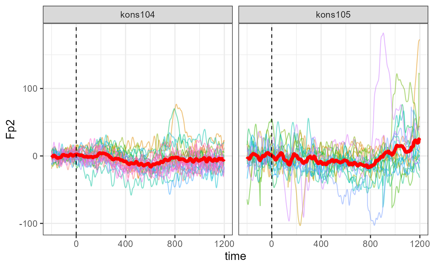
Other functions
ERP_to_times()
This function converts ERP List to dataframe with ERP components and time vectors.
times <- seq(-200, 1198)

ERP_dat <- ERP_to_times(ERPs, times)

print(ERP_dat)
#>       time      ERP
#>    1: -200 baseline
#>    2: -199 baseline
#>    3: -198 baseline
#>    4: -197 baseline
#>    5: -196 baseline
#>   ---
#> 1396: 1194 PostP600
#> 1397: 1195 PostP600
#> 1398: 1196 PostP600
#> 1399: 1197 PostP600
#> 1400: 1198 PostP600
get_markers()
Formats the vmrk files to extract information about markers:
marker_info <- get_markers("../inst/extdata/kons104_comp_BaselineCorrection_noncogn_incongr_nonviol.vmrk")
print(marker_info)
#>     descrip posit_datapoints marker_num posit_onset
#>  1:    S189                1        Mk2         101
#>  2:    S183              701        Mk6         801
#>  3:    S188             1401       Mk10        1501
#>  4:    S180             2101       Mk15        2201
#>  5:    S194             2801       Mk18        2901
#>  6:    S191             3501       Mk22        3601
#>  7:    S182             4201       Mk26        4301
#>  8:    S186             4901       Mk30        5001
#>  9:    S199             5601       Mk34        5701
#> 10:    S197             6301       Mk38        6401
#> 11:    S196             7001       Mk43        7101
#> 12:    S203             7701       Mk46        7801
#> 13:    S195             8401       Mk51        8501
#> 14:    S190             9101       Mk54        9201
#> 15:    S200             9801       Mk59        9901
#> 16:    S184            10501       Mk63       10601
#> 17:    S193            11201       Mk66       11301
#> 18:    S205            11901       Mk70       12001
#> 19:    S181            12601       Mk74       12701
#> 20:    S178            13301       Mk79       13401
#> 21:    S187            14001       Mk83       14101
#> 22:    S185            14701       Mk87       14801
#> 23:    S179            15401       Mk90       15501
#> 24:    S201            16101       Mk94       16201
#> 25:    S204            16801       Mk99       16901
#> 26:    S202            17501      Mk102       17601
#>     descrip posit_datapoints marker_num posit_onset
one_vhdr()
The BVA_to_R() function but for a single vhdr file:
file <- "../inst/extdata/kons104_comp_BaselineCorrection_noncogn_incongr_nonviol.vhdr"
path <- "../inst/extdata/"

one_vhdr(
  path = path,
  filename = file,
  sep = "_",
  ERP_list = ERPs,
  var_labs = c(
     "Subject", "Comp", "Export_Node",
     "Cognate_Status", "Congruency_Type", "Violation_Type"
  ),
  full_window_bounds = c(-200, 1198)
)
#>        time posit_datapoints    Fp2     F8    FT8     T8   TP8     P8   TP10
#>     1: -200                1 -5.132 -1.770 -0.219  2.732 4.565  9.213 -0.862
#>     2: -198                2 -4.047 -1.380 -0.543  1.518 3.966  8.941 -1.495
#>     3: -196                3 -2.915 -0.598 -0.586  0.341 3.340  8.509 -2.036
#>     4: -194                4 -1.929  0.565 -0.241 -0.690 2.540  7.840 -2.474
#>     5: -192                5 -1.137  2.049  0.470 -1.532 1.387  6.862 -2.753
#>    ---
#> 18222: 1190            18196 19.772 13.677 10.484 10.859 6.442 -0.628  2.124
#> 18223: 1192            18197 21.339 14.228 10.769 10.994 7.086  0.413  3.459
#> 18224: 1194            18198 22.281 14.521 10.731 10.918 7.539  1.227  4.723
#> 18225: 1196            18199 22.541 14.623 10.448 10.693 7.808  1.790  5.848
#> 18226: 1198            18200 22.054 14.579 10.006 10.363 7.880  2.095  6.715
#>           O2     Oz     O1    TP9      P7     TP7     T7    FT7     F7    FP1
#>     1: 5.375  1.354 -4.257 -4.016 -14.087  -9.069 -4.742 -2.709 -2.273 -2.221
#>     2: 5.183  0.686 -4.748 -4.816 -14.161  -9.707 -5.096 -1.484 -1.914 -2.004
#>     3: 4.824 -0.021 -5.079 -5.803 -13.910  -9.935 -4.933 -0.084 -1.125 -1.570
#>     4: 4.314 -0.713 -5.215 -6.734 -13.386  -9.775 -4.346  1.267  0.002 -0.953
#>     5: 3.662 -1.306 -5.088 -7.392 -12.635  -9.298 -3.473  2.356  1.351 -0.233
#>    ---
#> 18222: 0.223 -4.273 -0.775 -7.107 -10.039 -13.537 -7.029 -2.539 -0.039 14.938
#> 18223: 1.049 -3.848 -0.862 -5.942 -10.166 -13.272 -7.327 -2.937  0.572 17.343
#> 18224: 1.759 -3.299 -0.595 -4.504  -9.949 -12.758 -7.302 -3.222  0.703 19.413
#> 18225: 2.413 -2.581  0.021 -3.007  -9.448 -12.050 -6.992 -3.328  0.350 20.850
#> 18226: 3.107 -1.648  0.974 -1.635  -8.667 -11.141 -6.411 -3.141 -0.359 21.435
#>           AFz     F4    FC4     C4    CP4    P4     Pz      P3     CP3      C3
#>     1: -4.558 -7.670 -6.508 -7.184  0.137 5.398  3.268  -6.575  -2.973  -1.974
#>     2: -3.674 -6.318 -6.081 -7.493 -0.881 4.971  3.407  -5.853  -2.190  -0.900
#>     3: -2.402 -4.613 -5.246 -7.682 -2.129 4.117  3.333  -4.973  -1.258   0.424
#>     4: -0.918 -2.791 -4.202 -7.906 -3.652 2.822  2.982  -4.077  -0.305   1.794
#>     5:  0.646 -1.008 -3.099 -8.238 -5.452 1.139  2.343  -3.261   0.567   3.003
#>    ---
#> 18222: 16.521 18.660 21.484 13.345  6.427 5.928 -2.389  -8.759 -15.869 -16.665
#> 18223: 17.886 19.127 21.192 12.446  5.719 5.574 -3.198 -10.387 -17.758 -19.098
#> 18224: 18.712 19.045 20.381 11.318  4.979 5.273 -3.674 -11.398 -18.949 -20.843
#> 18225: 18.891 18.483 19.132 10.117  4.323 5.163 -3.757 -11.709 -19.319 -21.698
#> 18226: 18.412 17.532 17.562  9.010  3.872 5.343 -3.393 -11.246 -18.767 -21.512
#>           FC3     F3     Fz    FCz    CPz     Cz descrip marker_num posit_onset
#>     1:  0.263 -1.932 -3.884 -1.142  3.987  3.794    S189        Mk2         101
#>     2:  1.233 -1.061 -2.557  0.476  4.463  4.931    S189        Mk2         101
#>     3:  2.549  0.324 -0.682  2.514  4.854  6.143    S189        Mk2         101
#>     4:  3.980  2.005  1.466  4.651  5.037  7.242    S189        Mk2         101
#>     5:  5.314  3.724  3.666  6.611  4.915  8.039    S189        Mk2         101
#>    ---
#> 18222:  1.837  9.483 12.874 16.063  0.494  6.625    S202      Mk102       17601
#> 18223:  1.207 10.522 13.988 16.001 -1.074  4.815    S202      Mk102       17601
#> 18224:  0.500 11.151 14.454 15.360 -2.523  2.761    S202      Mk102       17601
#> 18225: -0.218 11.266 14.218 14.248 -3.655  0.700    S202      Mk102       17601
#> 18226: -0.840 10.851 13.323 12.797 -4.289 -1.109    S202      Mk102       17601
#>             ERP Subject Comp        Export_Node Cognate_Status Congruency_Type
#>     1: baseline kons104 comp BaselineCorrection        noncogn         incongr
#>     2: baseline kons104 comp BaselineCorrection        noncogn         incongr
#>     3: baseline kons104 comp BaselineCorrection        noncogn         incongr
#>     4: baseline kons104 comp BaselineCorrection        noncogn         incongr
#>     5: baseline kons104 comp BaselineCorrection        noncogn         incongr
#>    ---
#> 18222: PostP600 kons104 comp BaselineCorrection        noncogn         incongr
#> 18223: PostP600 kons104 comp BaselineCorrection        noncogn         incongr
#> 18224: PostP600 kons104 comp BaselineCorrection        noncogn         incongr
#> 18225: PostP600 kons104 comp BaselineCorrection        noncogn         incongr
#> 18226: PostP600 kons104 comp BaselineCorrection        noncogn         incongr
#>        Violation_Type
#>     1:        nonviol
#>     2:        nonviol
#>     3:        nonviol
#>     4:        nonviol
#>     5:        nonviol
#>    ---
#> 18222:        nonviol
#> 18223:        nonviol
#> 18224:        nonviol
#> 18225:        nonviol
#> 18226:        nonviol
Session Information
sessionInfo()
#> R version 4.0.3 (2020-10-10)
#> Platform: x86_64-w64-mingw32/x64 (64-bit)
#> Running under: Windows 10 x64 (build 17134)
#>
#> Matrix products: default
#>
#> locale:
#> [1] LC_COLLATE=Dutch_Netherlands.1252  LC_CTYPE=Dutch_Netherlands.1252
#> [3] LC_MONETARY=Dutch_Netherlands.1252 LC_NUMERIC=C
#> [5] LC_TIME=Dutch_Netherlands.1252
#>
#> attached base packages:
#> [1] stats     graphics  grDevices utils     datasets  methods   base
#>
#> other attached packages:
#> [1] ggplot2_3.3.2 BVAtoR_0.2.0
#>
#> loaded via a namespace (and not attached):
#>  [1] compiler_4.0.3    pillar_1.4.7      tools_4.0.3       digest_0.6.27
#>  [5] lattice_0.20-41   evaluate_0.14     memoise_1.1.0     lifecycle_0.2.0
#>  [9] tibble_3.0.4      gtable_0.3.0      pkgconfig_2.0.3   rlang_0.4.9
#> [13] rstudioapi_0.13   yaml_2.2.1        pkgdown_1.6.1     xfun_0.19
#> [17] withr_2.3.0       stringr_1.4.0     dplyr_1.0.2       knitr_1.30
#> [21] desc_1.2.0        generics_0.1.0    fs_1.5.0          vctrs_0.3.6
#> [25] systemfonts_0.3.2 rprojroot_2.0.2   grid_4.0.3        tidyselect_1.1.0
#> [29] glue_1.4.2        data.table_1.13.4 R6_2.5.0          textshaping_0.2.1
#> [33] rmarkdown_2.6     farver_2.0.3      purrr_0.3.4       magrittr_2.0.1
#> [37] scales_1.1.1      htmltools_0.5.0   ellipsis_0.3.1    assertthat_0.2.1
#> [41] colorspace_2.0-0  labeling_0.4.2    ragg_0.4.0        ini_0.3.1
#> [45] stringi_1.5.3     munsell_0.5.0     crayon_1.3.4      zoo_1.8-8